Saturday, June 2, 2018

EDGAR Data with requests and bs4

Edgar data with requests and bs4

THe SEC EDGAR archive is an immense store of structured data. There are afew libraries for accessing EDGAR and before evaluating them it seems like a good idea to try less specific tools. Below we use the requests and bs4 modules to pull a dataframe containing the CIK, company name, and location for an SIC.

Imports

In [14]:
# imports
import pandas as pd
import requests 
from bs4 import BeautifulSoup
import time

# CONST
SIC = 6189 # the sic searched for later
PAGEMAX = 100 # max entries per page available at this facility
URL = "https://www.sec.gov/cgi-bin/browse-edgar" # base url
REQL = ["company=", "match=", "CIK=", "filenum=", "State=" \
        , "Country=", "SIC=%04d", "owner=exclude", "Find=Find+Companies" \
        , "action=getcompany", "count=%d", "start=%d"] 
print("imports done")
imports done

pulling a single page

We can pull a single page with a url like the string below. This was modeled after the url from a browser session.

In [16]:
# reqS = "&".join(REQL)  %(SIC, 100, 0)
reqS = "?".join((URL, "&".join(REQL) %(SIC, 100, 0)))
reqS
Out[16]:
'https://www.sec.gov/cgi-bin/browse-edgar?company=&match=&CIK=&filenum=&State=&Country=&SIC=6189&owner=exclude&Find=Find+Companies&action=getcompany&count=100&start=0'

Obtaining the table with requests, and finding the table with bs4

In [19]:
respS = requests.get(reqS).content.decode() # do search
soup = BeautifulSoup(respS, "lxml") # pull into bs4 structure 
table = soup.findAll('table')[0] # find 0th table in bs4 structure 
respDF = pd.read_html(str(table), header=0)[0] # get 0th dataframe from table 
respDF.head()
Out[19]:
CIK Company State/Country
0 1738503 20 Times Square Trust 2018-20TS NY
1 1715687 280 Park Avenue 2017-280P Mortgage Trust NY
2 1740866 5 Bryant Park 2018-5BP Mortgage Trust NY
3 1053428 A I RECEIVABLES CORP NY
4 1094412 A.I. RECEIVABLES TRANSFER CORP. NJ

Function to grab pages till there are no more pages

In [21]:
def getSIC(sic, url=URL, pagesize=PAGEMAX):
    """
    pull dataframes from url till they are empty,
    then concat and return
    """    
    dfL = []
    while 1:
        time.sleep(1)
        reqS = "?".join((url, "&".join(REQL) %(SIC, pagesize, pagesize*len(dfL))))
        try:
            respS = requests.get(reqS).content.decode()
        except:
            break
        soup = BeautifulSoup(respS, "lxml")
        try:
            table = soup.findAll('table')[0]
        except:
            break
        respDF = pd.read_html(str(tableL[0]), header=0)[0]
        dfL.append(respDF)
        if len(respDF) == 0:
            break
    return pd.concat(dfL)

Calling function and checking on it's length.

In [25]:
testDF = getSIC(SIC)
testDF.shape
Out[25]:
(11600, 3)
In [23]:
testDF.head()
Out[23]:
CIK Company State/Country
0 1738503 20 Times Square Trust 2018-20TS NY
1 1715687 280 Park Avenue 2017-280P Mortgage Trust NY
2 1740866 5 Bryant Park 2018-5BP Mortgage Trust NY
3 1053428 A I RECEIVABLES CORP NY
4 1094412 A.I. RECEIVABLES TRANSFER CORP. NJ

Monday, May 28, 2018

Using requests Module to Search FRED Metadata

notr

FRED data with requests

The FRED API is so easy to use that finding what series to read is the hard part. There are hundreds of thousands of series, too many even to list in a simple html table. API calls through the requests module can help.

For pulling individual series, we do not need an API key, so it's simple for anyone to copy a notebook and follow along. For pulling metadata, a key is required. There is a key in the notebook.

So many FRED sequences have non-farm descriptions that it made me wonder what series they have for farms, so we take a look at that.

Imports

In [31]:
# imports
import pandas as pd
import requests 
import json 

# CONST
fredKey = "see notebook" # api key for notebook

requests.get

The requests.get method takes a string argument. The string has the following components connected with anpersands

  • base tags search url and tag to look for
  • api key
  • file_type=json

The decode method for the content attribute from that output is a json string we'll interrogate.

In [18]:
reqS = "&".join(("""https://api.stlouisfed.org/fred/tags/series?tag_names=%s
api_key=%s
file_type=json""" %("farm", fredKey)).split("\n"))
respS = requests.get(reqS).content.decode()
len(respS)
Out[18]:
573397

The string from the request can be sent to json.loads to obtain a dictionary.

In [32]:
tD = json.loads(respS)
tD.keys()
Out[32]:
dict_keys(['realtime_start', 'realtime_end', 'order_by', 'sort_order', 'count', 'offset', 'limit', 'seriess'])

It's the "seriess" entry we are interested in, and that is a list of dictionaires.

In [33]:
seriesL = tD["seriess"]
len(seriesL)
Out[33]:
838

So there are over 800 series with "farm" in the tags. Just browsing one shows a dictionary.

In [34]:
seriesL[0]
Out[34]:
{'frequency': 'Annual',
 'frequency_short': 'A',
 'group_popularity': 1,
 'id': 'A0282AUSA398NNBR',
 'last_updated': '2012-08-16 11:38:36-05',
 'notes': 'Series Is Presented Here As 3 Variables: (1) Original Data, 1915-46; (2) Original Data 1946-63; (3) Seasonally Adjusted Data, 1939-46. Included In This Series Are: (1) New Housing Units And Additions And Alterations To Existing Units On Places Classified As Farms, According To The 1960 Census Definition; And (2) Other Buildings And Structures Used In Farm Production, Such As Barns, Storage Houses, Smoke Houses, Fences, Wells, Etc. Excluded Are Operations Which Are An Integral Part Of Farming, Such As Plowing, Terracing, And Digging Of Drainage Ditches. For Further Information On Sources, Collection Procedures, And Coverage, See Introductory Notes On Bls-Dept. Of Commerce Series, And Lipsey & Preston, Pp. 263-264. Source: Business & Defense Services Administration And Bureau Of Labor Statistics Publications (See Note).\n\nThis NBER data series a02182a appears on the NBER website in Chapter 2 at http://www.nber.org/databases/macrohistory/contents/chapter02.html.\n\nNBER Indicator: a02182a',
 'observation_end': '1946-01-01',
 'observation_start': '1915-01-01',
 'popularity': 1,
 'realtime_end': '2018-05-28',
 'realtime_start': '2018-05-28',
 'seasonal_adjustment': 'Not Seasonally Adjusted',
 'seasonal_adjustment_short': 'NSA',
 'title': 'Private Farm Construction for United States',
 'units': 'Millions of Current Dollars',
 'units_short': 'Mil. Of Current $'}

Sunday, May 27, 2018

FRED Data with pandas_datareader

FRED data with pandas_datareader

The Federal Reserve Bank of St. Louis publishes a lot of series and has a simple API. Below we take a really quick look at a couple of unemployment series. Really quick because it's just a couple lines beyond the expected imports.

Imports

In [2]:
# imports
import pandas as pd
from datetime import datetime as dt
pd.core.common.is_list_like = pd.api.types.is_list_like # workaround
import pandas_datareader.data as pdd
import matplotlib.pyplot as plt

# CONST
Sdt = dt(1990, 1, 1) # negative infinity date
Edt = dt(2020, 1, 1) # future date 
SW = "HSGS2564W" # Unemployment Rate - High School Graduates, No College, 25 to 64 years, Women
SM = "HSGS2564M" # Unemployment Rate - High School Graduates, No College, 25 to 64 years, Men

Grab data with DataReader

Arguments are

  • series wanted or a list of series wanted
  • constant "fred" to indicate we are reading from FRED. Could have supplied instead "google" for Google Finance, or "ff" for Kenneth French's data library
  • earliest datetime wanted
  • latest datetime wanted

There are some additional arguments not use here. For more details, help(pdd.DataReader).

In [3]:
# grab data
noCollegeDF = pdd.DataReader((SW, SM), "fred", Sdt, Edt)
noCollegeDF.head()
Out[3]:
HSGS2564W HSGS2564M
DATE
2000-01-01 3.8 3.7
2000-02-01 3.7 4.1
2000-03-01 3.5 3.8
2000-04-01 3.0 3.5
2000-05-01 3.5 2.9

Plot

In [4]:
%matplotlib inline  
fig, ax = plt.subplots() 
noCollegeDF.plot(ax=ax)
plt.title("Unemployment for HS Grads with No College W and M")
Out[4]:
Text(0.5,1,'Unemployment for HS Grads with No College W and M')

Tuesday, May 22, 2018

World Bank Data with pandas_datareader

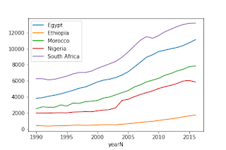
The World Bank publishes lots of data. They make data available for download as csv, xml, or xls files. Additionally, they make the data available through API calls, which is the civilized route. Tariq Khokhar wrote an excellent survey of libraries for accessing World Bank data in Python, R, Ruby, and Stata. We'll use one of the libraries discussed, pandas_datareader. This will be a quick look at per capita GDP trends for a few countries using pandas_datareader. In another blog post, we'll look at the same exercise using the csv files to show how much harder it is.

World Bank Data

Scanning the list of indicators, we see the link to "GDP per capita, PPP...", and the text for the link gives the indicator code we are looking for, "NY.GDP.PCAP.PP.CD". Additionally we can note from the chart that the populated data starts in 1990. Following the link, we get the option to download the series as csv, xml, or xls, and can download a file (now named API_NY.GDP.PCAP.PP.CD_DS2_en_csv_v2_9908727.zip, but it could be something else another day) to use in a later blog.

Installing pandas_datareader

A pandas_datareader can be installed using conda:

$ conda install -c anaconda pandas-datareader

Using pandas_datareader

The following can be downloaded as a notebook. The chart created in the notebook can be seen below.

world bank data with pandas_datareader

Downloaded ppp data csv. Workaround neded for version incompatability in datareader. See discussion</a href>.

In [33]:
# imports
import os
import pandas as pd
pd.core.common.is_list_like = pd.api.types.is_list_like # workaround
from pandas_datareader import wb as WB

# CONST
indCode = "NY.GDP.PCAP.PP.CD" # code for  per capita ppp gdp

Downloading with pandas_datareader

Arguments are

  • indicator= Code for series to grab
  • country= "all" or list of 2 byte country codes. Defailt is to "CA MX US".split(). We should prefer to filter in Python rather than in the pull.
  • start= Desired start year. Better to filter in Python so set early.
  • stop= Desired stop year. Better to filter in Python so set late.
In [50]:
# grab all data for 
pppDF = WB.download(indicator=indCode, country="all", start=1980, end=2020)
pppDF.head()
Out[50]:
NY.GDP.PCAP.PP.CD
country year
Arab World 2017 NaN
2016 16726.722185
2015 16302.363760
2014 15934.202070
2013 15548.200905

Reshaping the data

  • Removing rows with null entries.
  • Reseting indexes because you never want indexes.
  • Giving a normal whitespace free name to the series.
  • Sorting just to make table display read better.
  • Making numeric copy of the string year.
In [51]:
pppDF = pppDF.dropna().reset_index()
pppDF.columns = "country year GDPpc".split()
pppDF.sort_values("year country".split(), inplace=True)
pppDF["yearN"] = pppDF.year.apply(pd.to_numeric)
pppDF.head()
Out[51]:
country year GDPpc yearN
1263 Albania 1990 2722.280344 1990
1290 Algeria 1990 6616.408352 1990
1317 Angola 1990 2840.200763 1990
1344 Antigua and Barbuda 1990 10587.593409 1990
26 Arab World 1990 6759.785391 1990

Filtering for top African economies

The spelling of Egypt is a little unfortunate. Here we need exact matches.

In [52]:
# top Africa economies
aL = "Nigeria|South Africa|Egypt, Arab Rep.|Morocco|Ethiopia".split("|")
africaDF = pppDF[pppDF.country.isin(aL)]
africaDF.head()
Out[52]:
country year GDPpc yearN
2571 Egypt, Arab Rep. 1990 3819.286370 1990
2694 Ethiopia 1990 421.378824 1990
4261 Morocco 1990 2528.458556 1990
4514 Nigeria 1990 1965.827996 1990
5256 South Africa 1990 6267.091465 1990

plotting

In [54]:
# the next line is needed to diaplay the plot in the notebook
%matplotlib inline  
import matplotlib.pyplot as plt
fig, ax = plt.subplots() 
africaDF.groupby("country").plot(x="yearN", y="GDPpc", ax=ax)
ax.legend("Egypt|Ethiopia|Morocco|Nigeria|South Africa".split("|"))
fig.savefig("africaGDPpc.png")